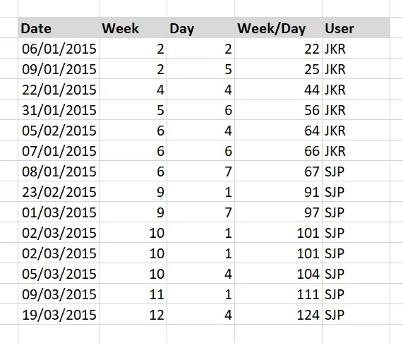
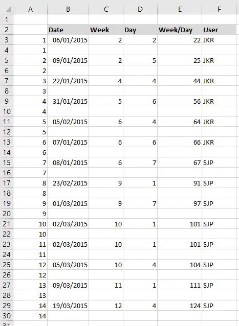
Hello, Excellers. Welcome back to another blog post in my #Excel 2021 series. Today let’s look at a really useful but very straightforward Excel tip. I will show you how to insert a blank row after every data row in your Excel worksheet. No formulas, not macros and no coding. Here a sample data set to work with below.
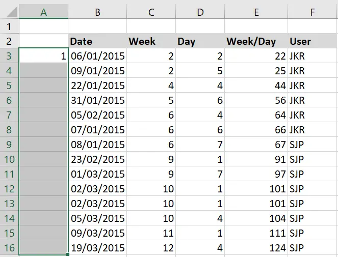
First a helper column is needed. So, if the data starts in Column A in the Excel worksheet insert a column to allow your data to start in Column B. Column A is going to be used for this helper column.
To start, type 1 in the first cell of your helper column. This should be in the first row of data. Avoid the header row. The next step is also easy highlight all cell in Column A to the bottom of your data set. My example is easy. It only contains 16 lines of data. Use the Excel shortcut Ctrl+Shift+Down Arrow to quickly highlight the full column of data if required.
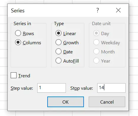
Next, use the fill series to fil the row numbers.
- Home Tab
- Editing Group
- Fill | Fill Series
- Complete the Step value (1 in this example)
- The stop value is the last rows of data (14 in this example)
- Hit ok. Excel fills the series accordingly.
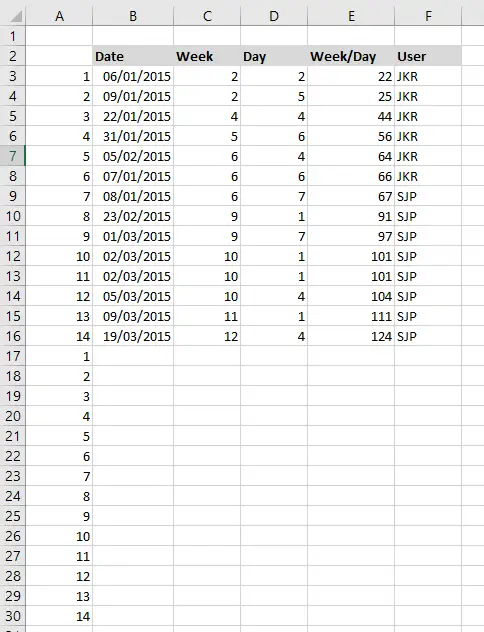
The final part of this tip is clever. Copy the Fill series from the steps above and past below the last row of data. This will be used to insert the blank row after each data row.
Finally, select the full data set.
- On the Home Tab go to the Editing Group.
- Sort and Filter.
- Sort Smallest To Largest.
- That is it job done. Each blank row is inserted.
- Delete the helper column.
