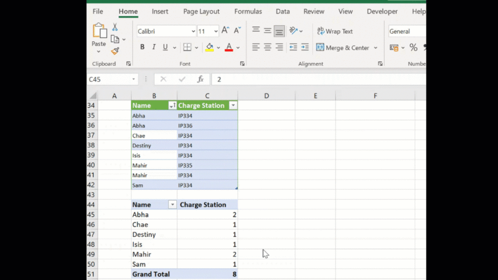
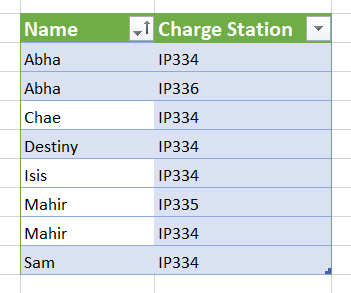
Hello and welcome to another blog post in my 2021 Excel tips series. This blog post is in response to a question by a subscriber. They wanted to use their Pivot Table to filter out duplicates in their data. So, in this simplified sample data set I have some employee records for allocations of charging stations. Some of the records are duplicated.
This a small sample replication of the data set. The original was a lot bigger. Also, there are MANY ways to identify duplicates in Excel. This is one of the ways. The user wanted to just use their Pivot Table records to achieve this. I hope you find it useful.
I will assume that you have your Pivot Table created. If you need some guidance on creating Pivot Tables you can watch my YouTube Video on creating your first Pivot Table. The link is below. I also have a great recommendation for a Pivot Table course. See that link also below.
Filter Or Show Duplicates.
Once you have your Pivot Table created, then add one of your fields to the values section. This calculation needs to be set to COUNT. It may default to SUM depending on the data type or other reasons. (See below for discussion on why that may happen).
The COUNT of values is required in this instance. Once that is done, use the value filter to filter duplicates or records greater than 1 (>1). Finally, those accounts with duplicate records are left.

How do you deal with duplicates in your Excel data?. There are a lot of methods. This is only one of man ways to filter duplicates

