Hello Excellers and welcome back to another #Excel tip in my 2019 series of #formulaFriday. Do you need to highlight expired dates? or any dates that are before the current date?. Well, this Excel tip will help you do that easily. In my example today I will show you step by step how to use the TODAY() function with some conditional formatting to highlight expired dates or dates before today. Let’s get started!.

Sample Data Set.

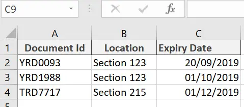
Here is my sample data set. I have an index or reference of paper records, their location and the date of expiry. These relate to records that need to be destroyed after the date of expiry is before the current day’s date.

So, I need to identify those records that require removing from my records section and destroy them.  I  will highlight the Expiry date, only if it is after the current or today’s date.  So, let’s get on with writing our formula to enable our conditional formatting.

Conditional Formatting Using A Formula.

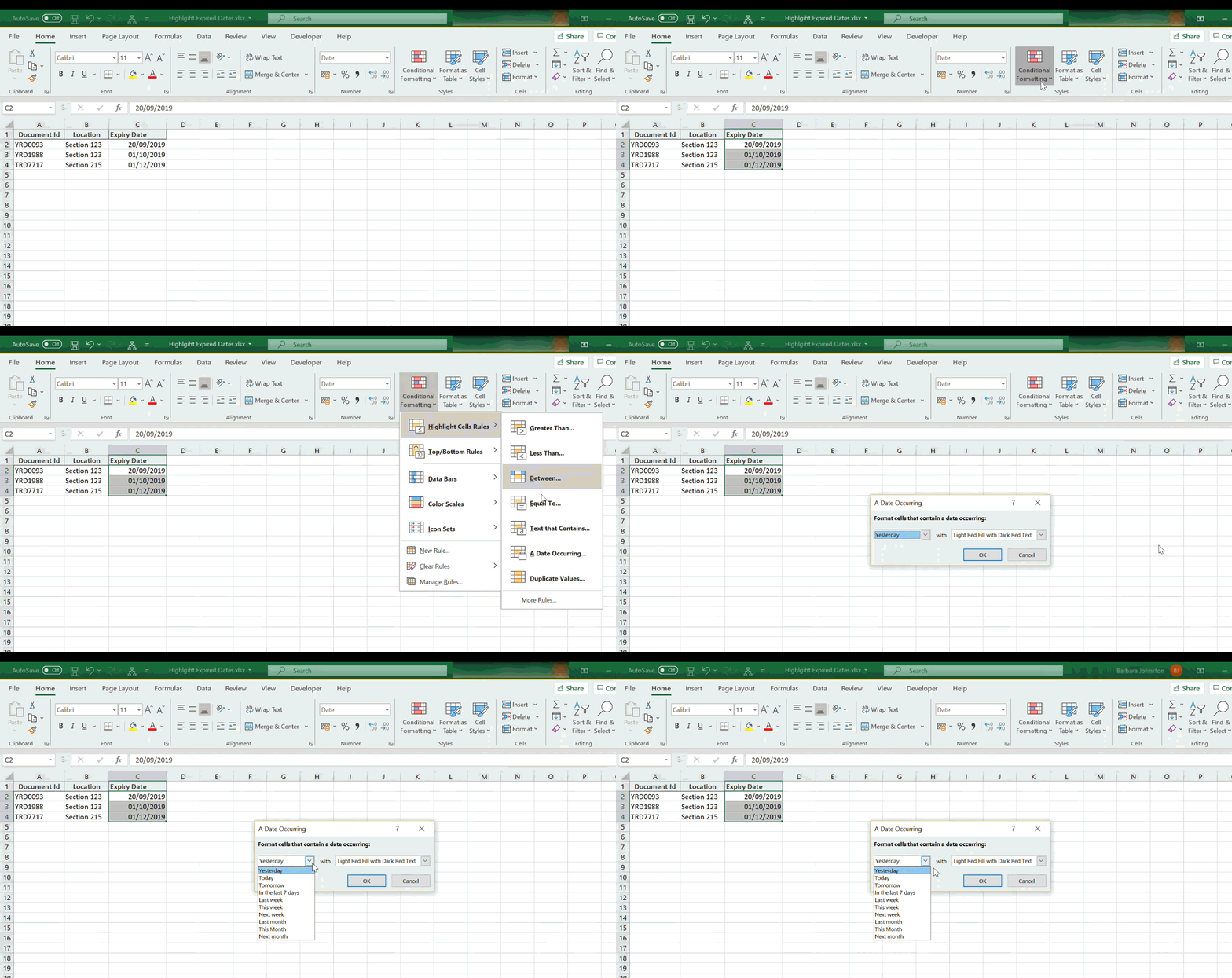
The solution we are going to use today uses a formula to set the conditional formatting rules. Now, Excel does come already packed with a stack of pre-defined rules to use. If you want to check them out then you can see them in the following location

Home Tab | Style Group | Conditional Formatting

As I want to test the condition before or equal to Today’s date I want to use a formula. This gives me more scope to decide my rules to conditionally format my cells.

The Today Function To Highlight Expired Dates.

The Excel TODAY function is simple. The syntax for a quick recap is as follows

=TODAY()

There are no arguments for the TODAY function. See, didn’t I tell you it was simple?. Once you type this function into Excel then today’s date is displayed. We can, therefore, use it in conditional formatting to test if the condition is TRUE or FALSE. This is how we conditionally format cells.

• Select the cells to conditionally format.
• Home Tab | Styles Group| Conditional Formatting.
• New Rule | Use a formula to determine which cells to format.
• In the Edit, Rule dialog box type the following formula

=C2<=TODAY()

• The final stage is to set your formatting. I have chosen a Red fill.

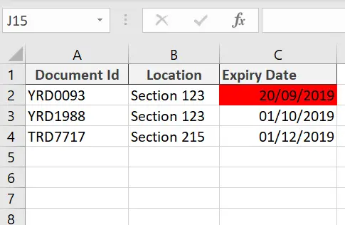
The result of my data set with the conditional formatting can be seen below.  Today’s date is 29 September so it has correctly conditionallty formatted record YRD0093.  I need to go to Section 123 and destroyt this record.

That’s it. it works i can now highlight expired dates in my Excel data set.

If you want more Excel and VBA tips then sign up to my monthly Newsletter where I share 3 Excel Tips on the first Wednesday of the month and receive my free Ebook, 30 Excel Tips.

Likewise, if you want to see all of the blog posts in the Formula Friday Series Click The Link Below.

How To Excel At Excel – Formula Friday Blog Posts.

So, Don’t forget to SUBSCRIBE to the How To Excel At Excel Newsletter for more tips the first Wednesday of the month. Just click on the link and enter your email. No spam. Just Excel tips.

Finally, I am delighted to let you know I have teamed up with Excel Rescue. Have you got a problem with Excel?. Get Help with Excel – Fast! Excel Rescue is a done-for-you small tasks service for Microsoft Excel. Why don’t you check out how they can help you. Click on the link below for special offers on Excel solutions. Book mark the link for furture reference.