Formula Friday - Use VLOOKUP With a Wildcard

Hello, Excellers and welcome back. It is Friday Formula time again. Today’s post will look at how to use wildcards in a VLOOKUP formula. Let’s begin with an example to demonstrate the method.

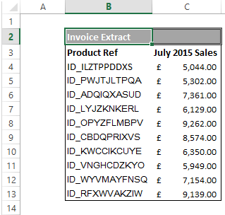
I have an extract of data that contain my invoice data. The extract is in CSV format from my accounting program. The data has some trailing characters to the right of the Product Ref data in Column B. We cannot readily see these in the raw data extract. But, it does have a huge impact when we try to do any analysis with the data.

Using A Standard VLOOKUP Formula

If I try to use a standard VLOOKUP to match the Actual Sales Value with my Target Sales sheet, the formula appears to not work. It looks like I should be able to look up and find a match between these two data sets. If I look at the Product Ref fields, they do appear to look exactly the same. The issue is my trailing spaces that are considered true characters by Excel. They are not in my Sales Targets sheet values. So, the two sets of Product Refs are not the same. Excel, therefore, cannot find a match in the VLOOKUP formula.

See the result of trying the regular VLOOKUP below in this screenshot.

What Is The Solution?

I could use the TRIM function or numerous other formulas to clear of the trailing spaces. That would be useful if I knew exactly where they were in the data. There is one easier and quicker method is the use a wildcard with my VLOOKUP formula which will easily take into account any extra characters at the end of my Product Ref data field.

What Are WildCards In Excel?.

There are three types of wildcards in Excel. They are the ASTERIX(*), The QUESTION MARK(?) and the TILDE(~).

ASTERIX(*) – This represents any number of characters. For example, Ex* could be Example, Excel, Extreme etc.

QUESTION MARK(?). This represents one single character. For example, Tr?ck could represent Trick or Track.

TILDE(~). This is used to identify a wildcard character. What does this mean?. It is probably easier to explain with an example. Let’s say you want to find the exact phrase Happy in a list. If you use Trash* as the search string, it would give you any word that has Trash at the beginning followed by any number of characters (such as Trashy, Trashed). To specifically look for Trash, we need to use ~. So our search string would be Trash~*. Here, the presence of ~ ensures that excel reads the following character as is, and not as a wildcard. See how this works?.

We can now use CONCATENATION (&) to join our lookup value with the wildcard character as you can see below- (if you want to read more about CONCATENATION then see my corresponding post here).

=VLOOKUP(E4&”*”,$B$2:$C$13,2,FALSE)

Here is the formula explained

E4&”*” is the lookup value, the value in E4 and the * wildcard.
$B$2:$C$13 is the lookup range, the exported data, it is a locked down or absolute data range as I want to drag the formula down the column.
2 the column that has the value to return, the amount
FALSE tells the function to perform an exact match

See what happens when we use this wildcard in our formula.

Success! Our VLOOKUP is returning the expected result. The extra spaces after the Product Ref in my data extract have been dealt with easily by my use of the wildcard.

Have you used wildcards in formulas? Share in the comments below.