Happy Friday Excellers Welcome to another blog post in my Excel #formulafriday series. . Today let’s look at creating a search bar right in an Excel cell in our workbook. Yes, you can use the search function in Excel to create a dynamic search bar right in an Excel cell on your worksheet.so.
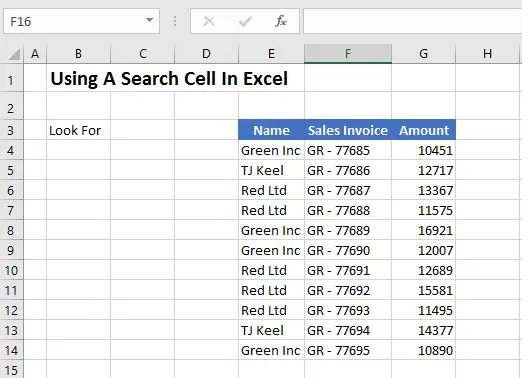
So, let’s work through an example. Here is my sample data set.
I have a shortened list of Sales Invoices. I want to use the Cell C3 as a search cell. Subsequently, I want Excel to highlight all of the cells in the data set that match the value that is in Cell C3.
We do this with Conditional Formatting, and using a formula to determine which cells to format.
Conditional Formatting Process.
- Home Tab
- Styles Group
- Conditional Formatting
- Use A Formula To Determine Which Cells To Format
The Search Function In Excel. Syntax Recap.
The formula is simple. THE SEARCH Function has 3 arguments
- find_text – The text to find.
- within_text – The text to search within.
- start_num – [optional] Starting position in the text to search. Optional, defaults to 1
So in our example, we are searching for the text in $C$3 in range starting in E4, we can leave the optional argument start_num so it defaults to 1. If the text in $C$3 is found in E4 then the condition is TRUE, the formatting is applied. Simple.


