Friday Formula Fun Time…..
Do you find that your VLOOKUPS are sluggish sometimes when you are dealing with larger data sets?. Here is a way to speed them up….use 2 VLOOKUPS at a time…..What?…. read on.
(If your Excel performance is good then this method is not really necesary but it is handly to know for those time you need it).
When you use a VLOOKUP in Exact mode. (i.e you are looking for an exact match in your data), Excel may have to look through 10,000, 50,000 or even 100,000 records individually to see those records that are a match. An exact match is specified in the fourth argument of the VLOOKUP formula.
Let’s take a reminder of the syntax of the VLOOKUP formula.
=VLOOKUP(lookup_value,table_array,col_index_num,[range_lookup])
Where
- Match = What you want Excel to find
- Table Array = Where you want Excel to look for it
- Column Number = If Excel finds it, how many columns from the left is the data you want?
- Range Lookup = Optional hence in the brackets, False= Exact Match, True= Approximate Match
So, when we specifiy FALSE as the Range Lookup where we want an EXACT match Excel goes through every single record, it can be slow, it is carrying out a linear search.
If we specify TRUE as the Range LOOKUP, where we will take an APPROXIMATE match Excel performance a LOT LOT faster. To use approximate-match VLOOKUP, you must sort your data by the first column (the lookup column). SO is this the answer then?, use the APPROXIMATE match argument. Unfortunately not. …
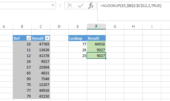
VLOOKUP won’t display an error if the lookup value doesn’t exist, and the result may look completely normal, even though it’s totally wrong as if the lookup value doesn’t exist. It will return the nearest match it can find. See in my example below. The Ref 25 does not exsit so Excel returns the details of the nearest match it can find – 24.

So what is the solution?. Exact match is uber slow and Approximate is fast but may not give the result we want?
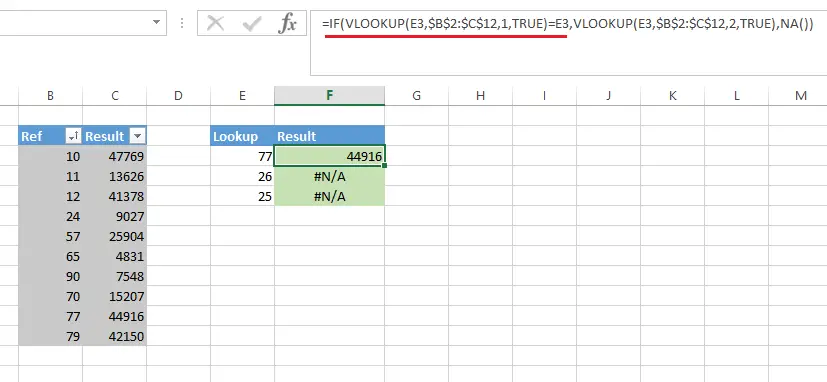
We can use VLOOKUP twice, with both of them using the approximate match!!. Let’s see how it works. The formula looks like this…..

The first instance of the VLOOKUP simply looks up the lookup value (in Column E in our example).
Excel returns TRUE only if the value is found. If the value is found then the second VLOOKUP runs and will return the matching value from our data table. If the lookup value is not found, then the ‘if FALSE’ part of the IF Formula runs and you can get Excel to return any value here you want.
In our example here I have decided to get Excel to return #N/A if a match is not found. 25 and 26 do not exist in our data set. Try this with a large data set and see if the performance of your VLOOKUP improves…let me know in the comments below.
Remember: to data by lookup value in order for this cool Excel trick to work.

YouTube Video- Create Your First Pivot Table
Fast Fun Way To Learn Excel Formulas
