Hi Excellers, it is time for another #formulafriday Excel article. Did you know that Excel has a SEARCH function? Most Excel users know the FIND Function, but what about SEARCH?. In Excel, the SEARCH function allows you to search for the location of a specific text string within another string. Here is a quick recap of the syntax of the SEARCH function.
Syntax Of The Search Function In Excel.
The syntax of SEARCH is relatively simple.
=SEARCH (find_text, within_text, [start_num])
- find_text – The text to find.
- within_text – The text to search within.
- start_num – [optional] Starting position in the text to search. This is optional, defaults to 1.
SEARCH returns the position of the first character of find_text inside within_text. Points to note, unlike the FIND function, SEARCH allows wildcards and is not case-sensitive.

How SEARCH Function Works.
Search allows us to find the location of text within a text string, and will return the number representing the location of the text.
Or in plainer words…..find the location of my text or text string within a cell containing text or a text string starting at the position I specify. A couple of great features it has is it’s NOT case sensitive and you can use wildcards with it. (Unlike the FIND Function)
A Working Example Of SEARCH.
Lets’ take a look at the basics then move on and see how useful it really can be. Here are the basics, with the formula showing in the result cell.
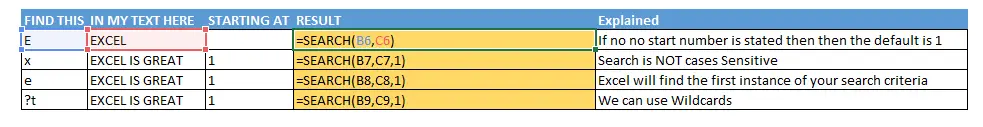
.This is the result of Excel’s calculation.

That’s cool right?, but let’s turn up the volume on this and use SEARCH to highlight any cells in my worksheet that contain the word “Store”.
Let’s say I have a data source I need to cleanse, and one of the issues I have is that there are many combinations of the word “Store”. This string could be present in differing cases, both upper and lower of even a combination of them both in my data source.
Being able to use Formulas within Conditional Formatting gives us infinite possibilities and flexibility. So all we need to do is get the formula to return TRUE when a cell contains “Store”.
- Highlight the cells that you want to condtionally format
- Home Tab
- Styles
- Conditional Formatting
- New Rule
- Use A Formula To Determine Which Cells To Format
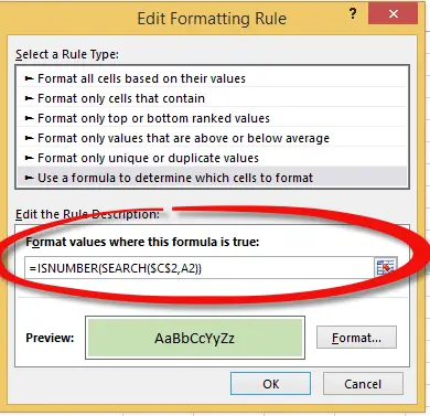
- In the formula dialog box type the following formula
- Choose how you want to format or highlight your cells, in my case I have chosen green
- Hit Apply
- Job Done
The formula uses SEARCH to find the position of the word Store and if that exists then it returns the position of it, andalso generates an error if it does not exist. But by encasing this in the ISNUMBER Function we can ignore the error and get Excel to return TRUE when a number is found, and then use this TRUE as a trigger to conditonally format the cell that contains Store.
When you apply conditional formatting using a formula, that formula is calculated relative to the active cell in that selection, and therefore the A2 will change to the address of the cell being evaluated, since A2 is relative. I have used $C$2 as an absolute reference to supply the Excel formula with the string I want to search for.
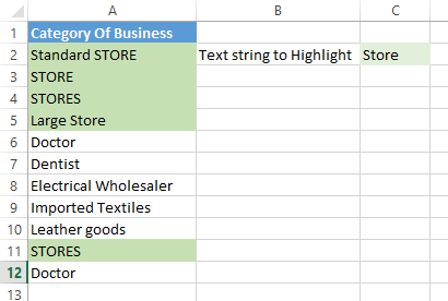
Success! No issues here. Job has been done.
More Excel Articles.