Happy Friday Excellers…..

Pivot Tables are great for taking hundreds or even thousands of rows of data and be able to summarise and analyse your data set with a few clicks of your mouse, if you want to read more about creating your first Pivot Table the you can check out my blog post here or my YouTube Video here.

Using A Dynamic Data Source

So, if you continually add extra rows to your Pivot Table data source, or indeed remove them it would be really useful to have Excel automatically adjust the data source to accommodate these changes. There are a few ways to create a dynamic data source, but today let’s look at using a dynamic formula to define a Named Range as the data source. Let’s go ahead and create it.

The Syntax of OFFSET Formula is-

reference – this argument is required it is the reference from where you want to base the OFFSET. This must refer to a cell or a range of adjacent cells.

rows – this argument is required it is the number of rows either up or down that you want the left uppermost cell to refer to.

columns – this argument is required it is the number of columns, left or right that you want the upeermost cell to refer to.

height – this argument is optional and is the height in the number of rows that you want the returned reference to be – it must be a positive number.

width – this argument is optional and is the width in the number of columns that you want the returned reference to be -it must be a positive number.

This example uses Excel 2013.

• Formulas Tab – Defined Names Group- Define Name
• In the New Name dialog box, call the named range something, I have called this range “my_data_range”.
• In the Refers To section is where we enter the OFFSET Formula, which returns a reference to a range specified by number of rows and columns.

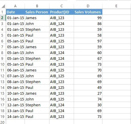
I have my sample data set below which is four columns in width- so I need to design a dynamic range which is four columns wide.

The arguments in this OFFSET formula are-

=OFFSET(Sheet1!$A$1,0,0,COUNTA(Sheet1!$A:$A),4)

The data is contained Sheet1

• Reference Cell -Sheet1!$A$1 – as this is a Pivot Table, we need the Column Names so we start at reference A1
• Rows to offset -0
• Columns to offset – 0
• Number of rows –COUNTA(Sheet1!$A:$A)
• Number of columns -4

The COUNTA part of the formula counts the number of values in the range that are not empty. We use this in the ROWS argument. When you add a value to the range i.e a new row of data, COUNTA($A:$A) increases. As a result, the named range expands. (Or reduces as rows are deleted) Cool huh?!.

There we have a dynamic range for our Pivot Table.

So, we need to do now is use the named range “my_data_range” as the data source for our Pivot Table.

You can download the example workbook to work through the OFFSET formula here.

[ddownload id=”9289″]

• Create A Timestamp In Excel
• Hide all of your Excel formulas from prying eyes!
• Undertand and debug Excel formula errors
• How To Display a Plus + Sign On Positive Numbers With Custom Formatting In Excel