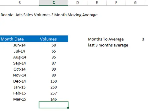
Hello Excellers and welcome to another #Excel #FormulaFriday blog post in my 2021 series. Today I want to share how to calculate a rolling or moving average in Excel. Calculating moving averages can be a really useful way to look at trends in data. For example, I want to know the last 3 months average sales of my Beanie Hats. I always want to analyze the last or latest three months, even when my new monthly sales data is added into my spreadsheet. I, therefore, need the calculations to move along to accommodate the new data that is automatically entered into my data set. The key to this is to use the Excel OFFSET function.
So, it is really easy to set up a formula in Excel to ALWAYS look at the 3 or 6 or any numbers of months in your data. Let’s take a look at an example.
Calculating A Moving Average.
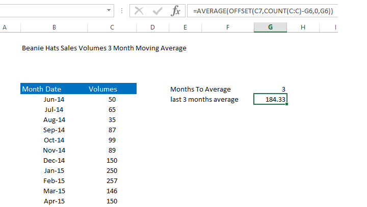
I have entered the number of months I want to use for the moving average in cell G6 in my example screenshot below. In this way, I can easily change the number of months I want to look at in my formula. I might at some point want to look at 6 months or 9 months. In which case I can simply change this number to the number of months to analyze.
The formula in G5 reads as below:-
=AVERAGE(OFFSET(C7,COUNT(C:C)-G6,0,G6))
Let’s break this down and work out what Excel is doing in this calculation.

Using the OFFSET Function.
Bringing It All Together. Offet and Moving Average.


So, What Next? Want More Tips?
If you want more Excel and VBA tips then sign up for my Monthly Newsletter where I share 3 Tips on the first Wednesday of the month and receive my free Ebook, 30 Excel Tips and check out all of my Formula Friday Blog posts below.
How To Excel At Excel – Formula Friday Blog Posts.
Do You Need Help With An Excel Problem?.
Finally, I am pleased to announce I have teamed up with Excel Rescue, where you can get help with Excel FAST. Why not check it out?.


