Happy Friday…More #FormulaFriday Fun for you.  Today let’s look at how to always add the last 3 values in your data set.

This formua is one that I have used for always returning the sum of the last N values in a data set even when more values are added to the data on on ongoing basis making the data set larger.  In this example I will show you how to  return the last 3 months sales values on on ongoing basis without having to amend the formula.

Let jump in and get started with an example.  Here are my sales values for January 2015 to Ootober 2015 of Beannie Hats.  I have yet to add in November 2015 figures but I have them ready and verified to just add into the Excel worksheet.

Here is the data set.

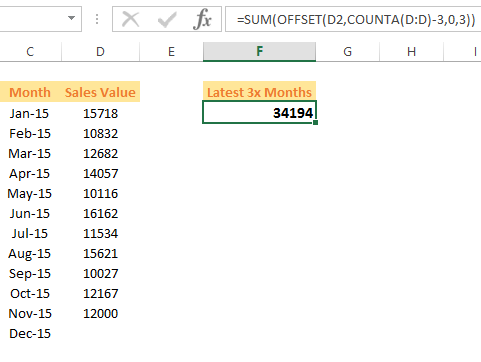
You can see I need to update the worksheet with November 2015 sales.  The formula to help me always have the latest 3 months figures is the following–

=SUM(OFFSET(D2,COUNTA(D:D)-3,0,3))

The SUM Function is taking the range reference provided by the OFFSET function to return the SUM value. We can focus on the OFFSET piece and walk through the formula.

 

The OFFSET function has the following syntax-

OFFSET(reference, rows, cols, [height], [width])

Reference this is our starting point or the the reference from which you want to base the offset.

Rows is the number of rows from the anchor point. Or the row offset.  A positive number means down from the anchor point and a negative number means up from the anchor point.

Cols is the number of columns from the anchor point, or the column offset. This number can be positive or negative.

Height Optional. The height, in number of rows, that you want the returned reference to be. Height must be a positive number.

Width Optional. The width, in number of columns, that you want the returned reference to be. Width must be a positive number.

So I can use the OFFSET Function within the SUM function….and let’s get back to the formula.

1. The first argument reference is D2 this is the starting point of our data set. ie. our Row 1 in our data set
2. The second argument rows is COUNTA(D:D)-3. This counts all non blank rows in Column D.  This plants us squarely at the row 10 in our data set -3 ROWS which navigates us to row 8 in our data set.  Note: It’s important not not have any blank cells in Column D as COUNTA will not return the correct number of rows to the argument.
3. The third argument cols is zero. We are not in this example off-setting left or right in the data set.
4. The fourth argument is 3.  We want to take the reference from the second row argument and count down 3 rows.
5. The fifth argument width is not used because we only want one column for the range.

So let’s go ahead and test it by entering in the sales figures for November 2015 which are 1200

Yes! Our sales figures are automatically updated with again to SUM the last 3 months.

You can download the example workbook for this tip here.

[ddownload id="8942"]

• View all of your Excel formulas at once
•  Hide all of your Excel formulas from prying eyes!
• Undertand and debug Excel formula errors
• Create A Timestamp In Excel Using Formulas