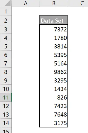
Hello Excellers, welcome to another blog post in my #Excel Tips, #FormulaFriday 2019 series. Today, let’s take a look at how to find the address of the cell that contains the maximum number in your Excel data set. Here is my sample data set to work with today.

Three Formulas To Solve This Excel Query.

To clarify, we actually will be using THREE formulas today to solve this Excel query. We will be using MAX to find the maximum value, MATCH to find the relative position of that maximum value in our data set or array. Finally, we will use the ADDRESS function to pinpoint the cell address of this maximum number. Ok, let’s kick this off by writing the first formula which is MAX.

Step 1. Use The MAX Function.

First, we need to find out what is the maximum value in our data set or array. This is really simple and straightforward with MAX. As a refresher, or if you are new to MAX the syntax of the formula is as below:

=MAX(number1, [number2], …)

• Number1, number2, … Number1 is required, subsequent numbers are optional. 1 to 255 numbers for which you want to find the maximum value.

In our example today the maximum value in our data set is 9862. The number array we use is in the cells B2 to B14.

Step 2. Use The MATCH Function With MAX

Next, we can use the MATCH function along with the MAX function. MATCH will give us the relative position of the MAX value within the data array. As with the MAX function, we can do a refresher, or if you are new to MATCH the syntax of the formula is as below:

=MATCH(lookup_value, lookup_array, [match_type])

The MATCH function syntax has the following arguments:

• lookup_value Required. The value that you want to match in lookup_array. For example, when you look up someone’s number in a telephone book, you are using the person’s name as the lookup value, but the telephone number is the value you want.
  
  The lookup_value argument can be a value (number, text, or logical value) or a cell reference to a number, text, or logical value.
  
• lookup_array Required. The range of cells being searched.
• match_type Optional. The number -1, 0, or 1. The match_type argument specifies how Excel matches lookup_value with values in lookup_array. The default value for this argument is 1.

So, in our example, the lookup_value is the value returned by our MAX formula. The result is 7 which is the relative position of the MAX value within our lookup_array.

Step 3. Using The Address Function.

Finally, we can take the ADDRESS function to return the actual address of a cell in a worksheet. The syntax of the ADDRESS function is as follows.

=ADDRESS(row_num, column_num, [abs_num], [a1], [sheet_text])

The ADDRESS function syntax has the following arguments:

• row_num Required. A numeric value that specifies the row number to use in the cell reference.
• column_num Required. A numeric value that specifies the column number to use in the cell reference.
• abs_num Optional. A numeric value that specifies the type of reference to return.

So as a result, in our example, the first argument or row_num if our combination of MATCH and MAX. The second argument specifies the column number.

Finally, we have the cell address of the highest or maximum value in our data set. This is useful if you have a very large set of data which can be difficult to navigate.

Have you used this method before?. Share in the comments below with other Excellers.

What Next? Want More Tips?

So, if you want more top tips then sign up for my Monthly Newsletter where I share 3 Tips on the first Wednesday of the month and receive my free Ebook, 30 Excel Tips.

 

 

A Full list Of Formula Friday Blog Posts

 

Do You Need Help With An Excel Problem?.

Finally, I am pleased to announce I have teamed up with Excel Rescue,  where you can get help FAST.