Adding a drop down list to your Excel sheet is a really great and convenient way to allow data entry to your Excel worksheets whilst maintaining good quality consistent data and reducing the amount of space taken up by lists!. If you want to review how to create a drop down list for data validation then check out my blog post here. So, if you are like me you possibly store a lot of hyperlinks in Excel?. They could be for reports, websites, data sources…you get the idea. I have all of my websites in one worksheet which is usually open all of the time.
So I am going to show you how to use the same drop down validation list to store Excel hyperlinks and reduce the amount of space taken up on your worksheet. (Real estate space is of a premium on a worksheet don’t you agree?) We will also insert a clickble cell to take you right to hyperlink destination.
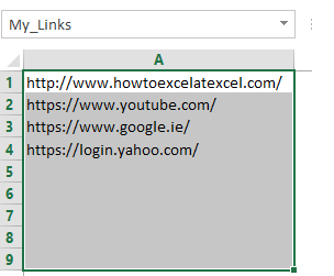
Its so simple to do. Here is my example. I have a named range called My_Links. They are stored on Sheet2 starting at cell A1.

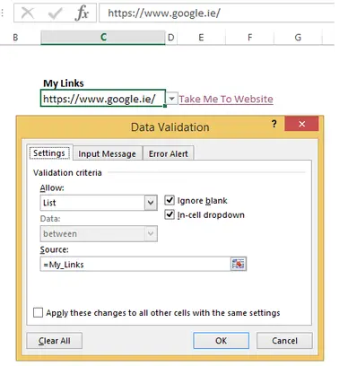
- Select the cell where you want your drop down list to appear. In my example it is in C4.
- Select data- Validation
- Data Validation Settings tab, select Allow: List, and make sure the In-cell dropdown box is checked.
- In Source ensure your range of cells (My_Links)
- Click Ok

- Select E4- this is where the clickable cell will be set up
- Finally, in E4 type the following =HYPERLINK(C4,”Take Me To Website!”) – type anything you want to.

So that’s it. A super easy way to create a drop down list for your Excel hyperlinks. Have you used this method before? Let me know in the comments below.
