Hello, Excellers and welcome back to another #Excel tip in my 2019 series of #FormulaFriday. Today, I will show you how to display the slicer selections of your Pivot Table in your Excel report title or header. This is a method I have used in a number of spreadsheet solutions and thought it would be a great tip to share.
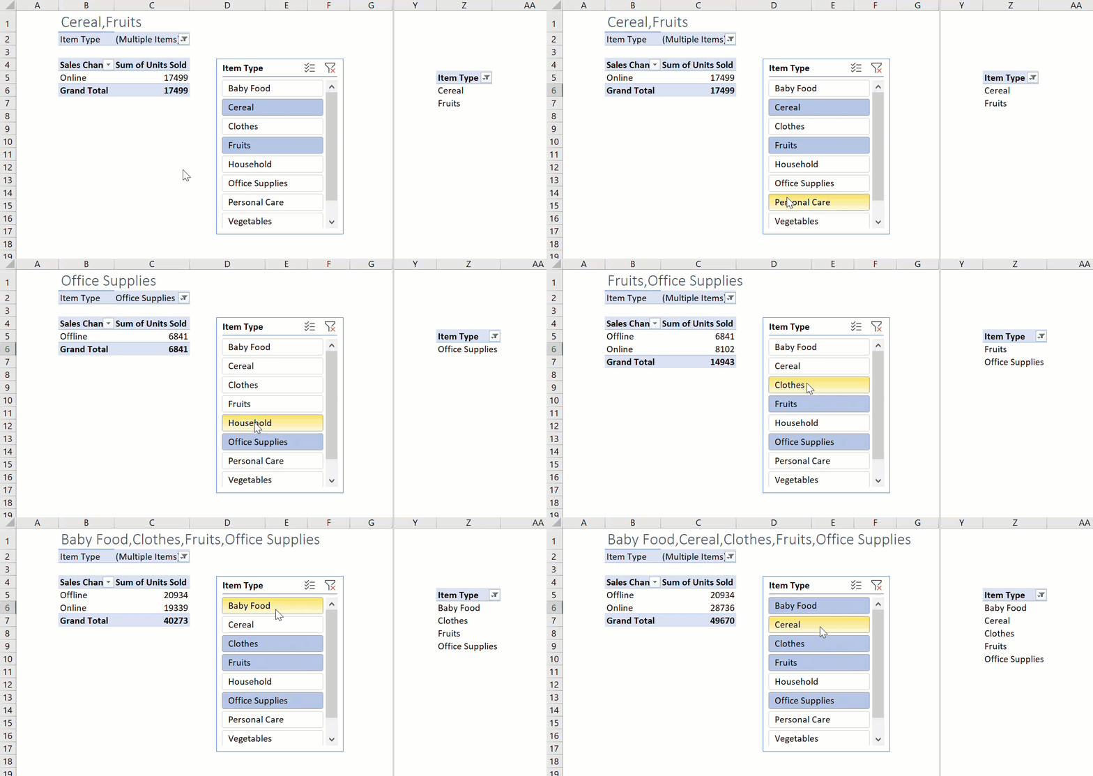
Now, let’s work through a simple example. I have created a simple pivot table with a sales data set, with Item Type as rows and the Sum of Units Sold in the data or calculation area. Pretty straightforward. You can see in the screengrab below I have the slicer selections displayed in cell B1.

This solution is especially useful if your selections are in the Filter area of the pivot table. Whilst it is easy enough to see the selections with the Item Type in the row area, if this were to move to the Filter position we can select one at a time and see the Item Type individually. But once more than one is selected we get the very (un)-useful Multiple Items display. You can see an example of this situation below once I select more than one item o filter.

Display The Excel Slicer Selections.
So, how exactly do you get the titles to appear.? Simply follow the steps below.
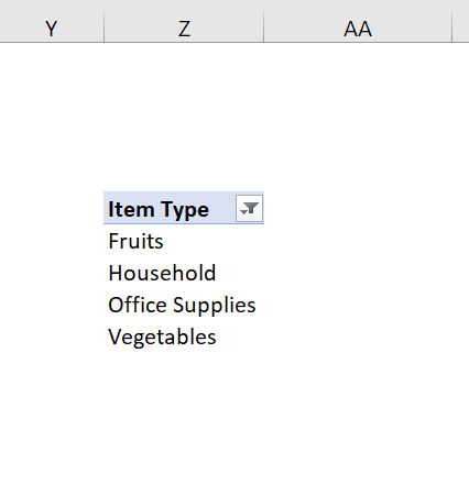
- Take a copy of your Pivot Table (your slicer should already be created) and place it out of view. In my example, I placed it in Column Z.
- To copy the Pivot Table in full – Place the cursor in the table | Pivot Table Analyze | Actions | Select | Entire Pivot Table | Ctrl+C to copy.
- Paste the Pivot in the out of view Column using Ctrl+V.
- In the pasted Pivot, place the slicer field – Item Type in this example in the rows area.
- Remove all other fields and values.
- Remove the Grand Total – Right Click | Remove Grand Total.

You will now be left with a list of Item Types in Column Z. Test the slicer by adding or removing Item Types. The list will grow or shrink as you select and deselect. Your slicer should be connected to this Pivot Table as well as your original. This is our list that we will use to populate the Report Header.
Using TEXJOIN To Create Report Headers.
Next, we will use the very useful TEXTJOIN function. This was introduced in February 2017 and it is a great addition to your Excel toolbox. Let’s get building our formula.
So, we now start the TEXTJOIN formula by typing = where you want to title to sit in your Excel worksheet. In this example it is B1.
TEXTJOIN has 3 arguments.
delimiter– this is the strong inserted between each text value. Usually a comma or space. In my example I am using a comma.ignore_empty – this argument if set to true will ignore any empty cells in the range of data to be joined. This is set to true as we can select the maximum number of cells that could contain the Item Types.
text1, text2, … text_n – this is the text to join. I will choose the range of cells that contain the Item Types in Pivot in Column Z.

So, all there is to do now if format the cell as a Title.
- Select the cell that contains the TEXJOIN function.
- Home Tab | Styles Group | Cell Styles | Titles and Headings.
- Select your preferred Style.
Now, all we need to do is test the solution. My favorite part!. Yes, it works.!. Finally, I can see my slicer selections in my report title.

What Next? Want More Tips?
So, if you want more tips then sign up for my Monthly Newsletter where I share 3 Tips on the first Wednesday of the month and receive my free Ebook, 30 Excel Tips.
 Finally, if you want to see all of the blog posts in the Macro Monday or Formula Friday Series, click on the links below
Macro Mondays Blog Posts.
Formula Friday Blog Posts.
Do You Need Help With An Excel Problem?.
Finally, I am pleased to announce I have teamed up with Excel Rescue, where you can get help FAST. All you need to do is choose the Excel task that most closely describes what you need to be done. Above all, there is a money back guarantee and similarly Security and Non-Disclosure Agreements. Try It!. Need Help With An Excel VBA Macro?. Of course, you don’t need to ask how to list all files in a directory as it is right here for free.


