Hi, Excellers welcome again to my #formulafriday blog post series. Today I want to share with you a great little hack for your chart axis labels. If you find yourself with a shortage of real estate on your dashboard or report (and let’s face it who doesn’t), then this little tip may just come to the rescue and free up a bit of space. Let’s take a look at using the CHAR() function.
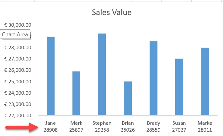
Take a look at my Excel chart below. I have created a chart where the x-axis labels INCLUDE the data value as well as the chart label. Cool huh?. Well, it really is easy the achieve this result with a few simple steps.
All we do is take advantage of the using the CHAR() function in a formula to generate the labels.
CHAR() Function Explained.
Syntax
The syntax for the CHAR function in is:
CHAR( ascii_value )

Where
ascii_value is the ASCII value used to retrieve the character.
Every character is Excel has an associated ANSI character code which determines what you see on your screen. The ANSI character set is 255 characters long numbered 1 to 255. An example being number 9 is character 57 and even the non-printing characters have codes assigned. Space is 32 and line break is 10. This is the one we are interested in.
If you want more Excel and VBA tips then sign up for my Monthly Newsletter where I share 3 Tips on the first Wednesday of the month and receive my free Ebook, 30 Excel Tips.
If you want to see all of the blog posts in the Formula Friday series. Click on the link below
How To Excel At Excel – Formula Friday Blog Posts.
Do You Need Help With An Excel Problem?.
I am pleased to announce I have teamed up with Excel Rescue, where you can get help with Excel FAST.


