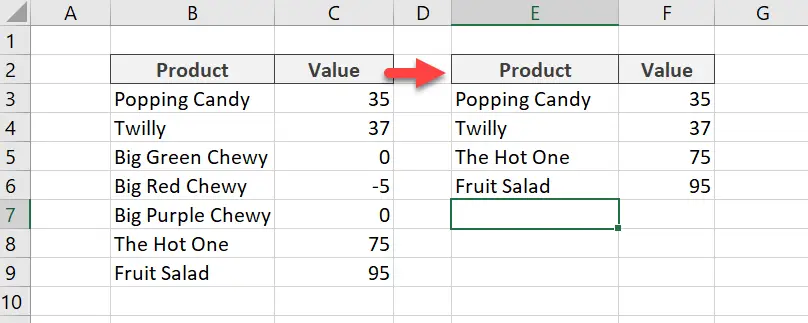
Hello Excellers and welcome to another Excel Tip in my #macromonday 2019 series. Today let’s look at how to copy cells based on specific criteria in your Excel worksheet. This is a macro I created to help speed up a repetitive process at work. I needed to copy and paste cells that were greater than zero. Specifically, all products that had a value greater than zero next to them. You can see a sample of similar data and my expected outcome from my Excel macro.

All of the rows with values in Column C have been copied to another area of my worksheet. Exactly what I need. So let’s get writing some VBA code right.

Preparing To Write The Macro

First, we will need to open the Visual Basic Editor.  There are two ways to do this.  Either by hitting ALT +F11 or selecting the Developer Tab | Code Group | Visual Basic.  Both methods have the same result. We then have a choice. Either create a module to store your code either in your Personal Macro Workbook or alternatively in your current workbook.  What’s the difference?. If you save the macro in your Personal Macro workbook it will be available for use in any of my Excel workbooks.  So, if you store it in the current workbook then use is restricted to that workbook.

Learn More About Your Personal Macro Workbook (PMW)

If you want to read more about your Excel PMW then check out my blog posts below.

Macro Mondays -Creating and Updating Your Personal Macro Workbook

Why Is My Personal Macro Workbook Not Loading Automatically?

Macro Mondays – Create A Shortcut To Your Personal Excel Macro Workbook

Starting The Macro

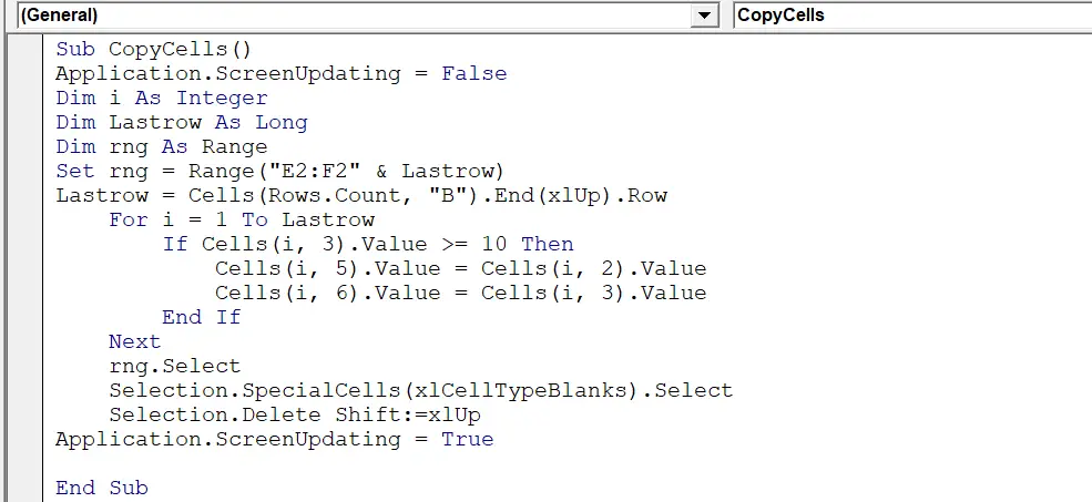
We need to start off the macro by inserting a New Module.  Do this by selecting the Personal.xlsb workbook, then Insert Module.  Type Sub then the name of the macro. In this example, I have called the macro CopyAboveZero. Excel automatically inserts the End Sub piece of code for us which ends the Sub Routine. So, all we need to do is insert the rest of the code.

[stextbox id=’info’]Sub CopyCells
End Sub[/stextbox]

Turn Off Screen Updating

By turning off screen updating we avoid the screen flashing or flickering as the Excel executes the VBA code. Any time a change occurs on your Excel worksheet, the screen will update.

[stextbox id=’info’]Application.ScreenUpdating = False
[/stextbox]

Declaring Variables

Next, we need to declare any variables we want to use in this macro. This just means that Excel allocates some memory to these values. We are also setting a range which represents the data in Columns E2 and F2 to the last row containing values.

[stextbox id=’info’]Dim i As Integer
Dim Lastrow As Long
‘Declaring variables
Dim rng As Range
Set rng = Range(“E2:F2” & Lastrow)

[/stextbox]

Finding The Last Row In Column A

We now find the last row in Column A. Probably like hitting the Ctrl+ Down arrow. This way we setting the cells that contain any values that we want to copy across our worksheet.

[stextbox id=’info’]Lastrow = Cells(Rows.Count, “A”).End(xlUp).Row
[/stextbox]

Use The For Next Loop With IF Then

The next stage is to use For…Next looping. Excel loops through to the last cell in Column B. It looks for cells which match our criteria which we have specified to be >= (greater than or equal to) 10. So, if these values are found then the code moves to the next stage of code.

In this case, the next stage is to show the value in the matching row in Column A in Column E. I also want to equate the cell values of Column C To Column F.

Excel continues to loop through all of the cells until all cells that meet the criteria have analyzed. Once all of the cells are completed the looping ends.

[stextbox id=’info’]For i = 1 To Lastrow
If Cells(i, 1).Value >= 10 Then
Cells(i, 5).Value = Cells(i, 2).Value
Cells(i, 6).Value = Cells(i, 3).Value
End If
Next
[/stextbox]

Remove Blank Cells.

I am now left with all of the correct data in Column E and F. My original data remains unchanged. The next stage is to remove the blank cells and move the data up to one complete new data set. By selecting the range set at the time we declared variables Excel will delete any blank cells and move our data to a neat complete data set.

[stextbox id=’info’]
rng.Select
Selection.SpecialCells(xlCellTypeBlanks).Select
Selection.Delete Shift:=xlUp
[/stextbox]

Turn Screen Updating Back On.

Next, we can turn screen updating back on after Excel has completed looping our code and deleting blank cells.

[stextbox id=’info’]
Application.ScreenUpdating = True
[/stextbox]

Ending The Excel Macro.

Finally, once all of the selected range has been checked for negative values the code finally ends. This instruction was already entered into the module for us when started the type the name of the macro.

[stextbox id=’info’]
End Sub
[/stextbox]

If you want more Excel and VBA tips then sign up to my monthly Newsletter where I share 3 Excel Tips on the first Wednesday of the month and receive my free Ebook, 30 Excel Tips.

Likewise, if you want to see all of the blog posts in the Macro Mondays Series Click The Link Below

How To Excel At Excel – Macro Mondays Blog Posts.

So, Don’t forget to SUBSCRIBE to the How To Excel At Excel Newsletter for more tips the first Wednesday of the month.