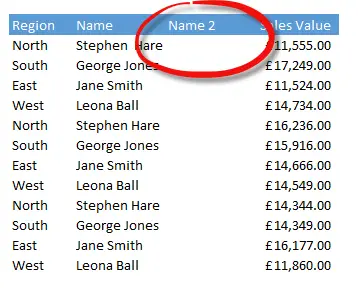
Have you come across a data set that looks a bit like this?. The source data in your Pivot Table is not as clean as it should be with a slight variation in spelling that is a right pain in the behind. This happens a lot to me and it is usually because my source data is coming from different data sources

Well, here is a really quick method for cleaning it up using TRIM.
TRIM removes all spaces from text except for single spaces between your words. It removes all spaces from text except for single spaces between words.
The Syntax of the TRIM formula is
=TRIM(text)
Where
text- Required. The text from which you want spaces removed
So let’s get this data cleaned up . First add a new helper column into your worksheet.

Type the TRIM formula into it like below.

Simply select your newly created column and hit Copy then Paste Special in the original column to replace your non cleansed data and then remove the helper column.
Now refresh your Pivot Table – Ta dah!. Your data is cleansed. Cool huh?.

