Download The Example Workbook Here
[ddownload id="7095"]
It’s Friday YAY. time for more Formula Fun….
Today let’s look at the LARGE function in Excel. It is a really handy one that will easily allow us to select a value based on it’s relative standing in your data set. For example to find the highest, runner up or 3rd place value in a a list of numbers.
The syntax of the formula is
=LARGE(ARRAY,K)
Where ARRAY = the range of cells that contains the data to be used in the function.
K= the Kth largest value such a the 3rd that is being south from the data.
Let’s look at an example with our data set as below which contains scores for a set of exam questions on a class. We will use the LARGE formula to find the score that is 3rd position in class based on the results of the exam.

- Select a cell to type your formula- in this case it happens to be H6
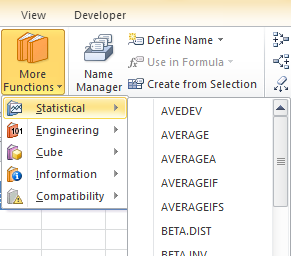
- Hit the Formulas Tab
- Select More Functions then Statistical to open the drop down list

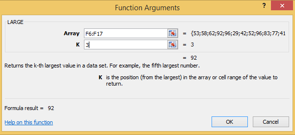
- Find LARGE and bring up the dialog box
- Click on the ARRAY- and highlight the cells in the scores list
- Click on the K line in the dialog box
- Type in 3 as we want to find the third largest – or third placed score
- Hit Ok

The answer is already in the dialog box which is 92. Once you hit Ok the result will be in G6.
We can then go ahead and repeat the process to find the highest ( 1st place) and 2nd place score.

So, the highest score in our data set is 99 and in second place is 96. Once you are familiar with the formula you can go right ahead and use the formula bar to type the formula straight into Excel.
Watch The Video
Want More Excel Formula Fun????

