Hello Excellers.  Welcome back to another #FormulaFriday #Excel blog post in my 2021 Excel series.  We all get them from time to time those Excel formula errors that annoy us and drive us nuts.  They also indicate to us that something is not working.  So, it useful to know.  Here is my guide to the main errors we seem to get and what exactly they mean.  Once we understand these formula errors we can avoid them or put them right.

Excel Formula Errors.

The #DIV!0 Error.

Simply means that you are trying to divide zero into a number.  For example

=B2/C2 would result in the #DIV/0! error if C2 contained zero.

You need to note that if the cell B2  was actually blank then Excel will also interpret that cell as containing a zero giving you equivalent as having the cell containing and actual zero.

How to fix the Error?

A simple piece of error handling looks after this one.

=IF(B2=0,0,B2/C2)

 The #Value Error.

This is probably the most popular error or should I say most frequently occurring. This error is displayed when the wrong type of argument or operand is used.

[An operand is simply items either side of an operator in a formula and these operands in Excel can be values, cells references, names labels etc.]

A quick example to explain

= B1*B2

If either of the cells above did not contain a number ie one contained a piece of text, then we would get the very popular #VALUE! error displayed.

 

How to fix the Error?.

Check your formula parameters have the correct data types in the above example B1 and B2 should contain numbers.

[This is why one should NOT change the default horizontal alignment of data cells. The text should always be always left-aligned while numbers are right-aligned by default. See my previous post here for more detail on the default formatting in Excel to easily tell what formatting your cells contain].

 

The #REF Error

In Excel the #REF! error refers to invalid cell references.  This occurs when a formula contains incorrect cell references.  This happens in the following scenarios.

• Any columns or rows containing data used in the formula have been deleted- usually accidentally!
• An actual formula has been copied or moved to another cell and the referencing is then incorrect.
• Data used in the formula has been moved to another location leaving the formula or function with incorrect referencing.

How to fix the Error?

Well- if the data has been deleted accidentally, use the Undo button to return it- you will be lucky if this is the only reason that you are getting the #REF! error.

• If your data cannot be reinstated or recovered this way then you will need to re-enter the data as well as adjusting the cell references if you need to, a bit more long- winded but it can be easily done.
• Adjust/correct the cell references for formulas that have been copied or moved.
• Adjust the cell references for the formulas for data that has been moved.

This will rectify your error and get you back on track!

The #NULL! Error.

This error occurs when two or more cell references are not separated correctly in a formula.

Or

The start and end points of cell ranges are not separated by a colon (:)

How to fix the Error?.

• Ensure you use a comma is correctly used to separate cells in functions e.g. = SUM(A1, A2, A3, A4)
• Take care that the start and end points of a range in a function are correctly separated by a colon ( : ) e.g. = SUM(D1:D4)
• Check that a mathematical operator, such as a plus or minus sign is used to separate cell references in a formula e.g.   = D1 + D2 + D3 + D4.

The #NAME Error.

This error is also quite a basic one, it just means that either

Excel cannot recognise the Function you  are using

OR

A custom function you are trying to use does not have that code within the workbook, this is often the case when you are using a function that needs to be added in via Add ins. E.g the Analysis Toolpak.

 

How to fix the Error?

It is also easy to fix this error.

• 1. On the Tools menu click Add-Ins.
• In the Add-Ins available list, select the Analysis ToolPak box.
• Click Ok.

The best way to ensure your function is recognised by Excel is to type it in lowercase.  If Excel recognises the function it will automatically convert it to upper case- neat huh?

 The #N/A Error.

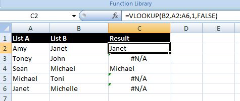
The most common reason for this error is when you are using LOOKUP Tables.  For Example, the VLOOKUP Function looks up column A for the value stored in B2 and returns a value if a match is found.  If the value that Excel is being told to look up is not found then the function returns the #N/A error.

 

How to fix the Error?

Well  you can ignore the error or get Excel to return ‘something else’ if the value its looking for is not found.  Let’s use an example, it’s always better to get some practice with formulas I find.

So in our example above, we have List A with our names and List B with the names to check are in List A, if we use the normal VLOOKUP formula then as we can see #N/A appears where we can’t find the corresponding names.

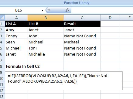
If we put a little addition to the VLOOKUP Formula in the way of the ISERROR function then we can get Excel to handle the error and display anything we want when the name isn’t found.

In this case I set it to tell me there was no name found. Great Stuff huh?

The #NUM Error.

This error occurs when Excel expects a number if a formula is expecting a number and you enter some text, or the result of your formula or function produces a number that is too large or too small for Excel to display.

 

How to fix the Error.

• Click the cell that displays the error, click the button that appears, and then click Trace Error if it appears.
• Review the possible causes and solutions.

So, I hope this helps with handling your Excel formula errors.  It really is important to know why your error is occurring and if it is ok to just skip, ignore or hide the error.

If you want more Excel and VBA tips then sign up to my monthly Newsletter where I share 3 Excel Tips on the first Wednesday of the month and receive my free Ebook, 30 Excel Tips.

 

So, Don’t forget to SUBSCRIBE to the How To Excel At Excel Newsletter for more tips the first Wednesday of the month.