 Welcome to Session 3 of Pivot Table Week.
In this session we are going to start getting some good information from our raw data, getting the Pivot Table to all of the hard work really start to Pump That Pivot For Data!
Just to quickly recap….
Session 1 we discussed what a Pivot Table is.
Session 2 we created out first Pivot Table.
As we already know from previous sessions the Pivot table is placed on a new worksheet and thats usually the best place for it. Specify in the Location box when prompted in the Pivot Table Wizard if you want to place it somewhere else.

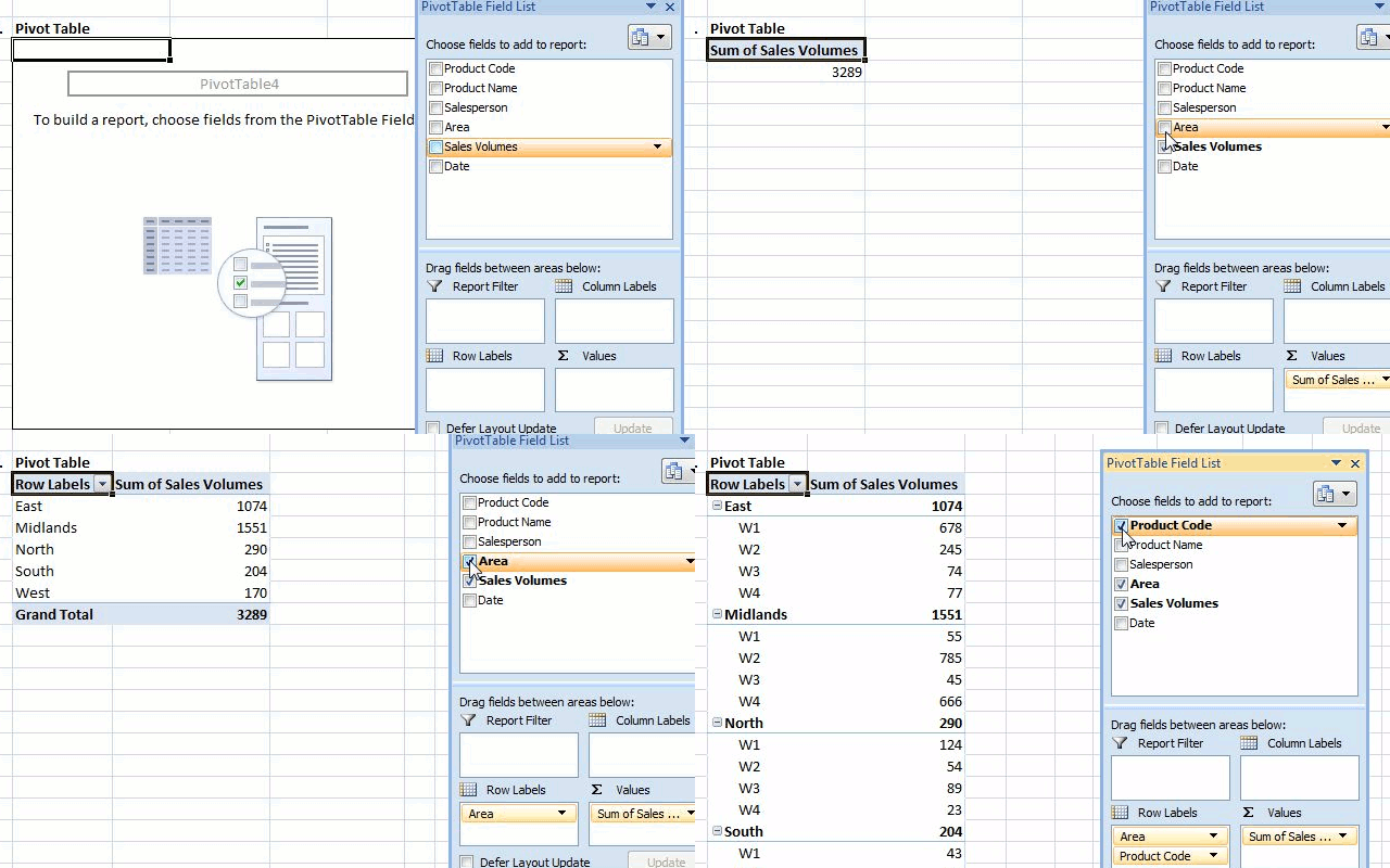
So, when your Pivot table is generated it is presented as a blank table on the left side of the worksheet and displays the Pivot Table Field List on the right hand side. The ROW and COLUMN labels boxes hold the fields that will appear on the row and column axes.
The report FILTER box holds the field or indeed fields hat you want to filter the table and the VALUES box holds the field or fields you want to use for your calculations ie the data you are summarizing, in this example it will be Sales Volumes.

The field list is docked at the right by default, feel free to undock it, drag it across the worksheet and place it wherever you want to.
So, to crunch some data all you need to do is select the check boxes for those fields in the ‘Choose To Add To Report’ of the Pivot Table Field List Window. As you add in fields Excel will position them in the four the numerous boxes which represent the various parts of the table.
If you don’t want the default table locations that Excel chooses then just move fields to the locations you want to by dragging them between the various boxes in the Pivot Table Field List Window.
In my example below lets look at
1. Total Sales By Area.
Let’s dig a little deeper and add in the Product Ref
2. Total Sales By Product Ref By Area
And futher
3. Total Sales By Product Ref By Sales Person
In this examples we can move the Sales Person along the Columns and the information looks a lot better.
Already we are getting some really good information out of our Pivot Table on the sales of Widgets.
Play Around with the Download Example you can download it here if you have not done so already.
{filelink=7}
See You For Session 4- Of Pivot Table Week where we discuss adding in some custom calculations to our Pivot Tables.


