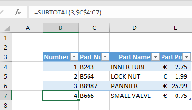
Hello Excellers time for some handy #formulafriday tips. This week let’s take a look at using the SUBTOTAL Function to easily number our rows in an Excel Table.
You may want to number the rows within the table itself instead of relying on the rows numbers in Excel on the left of the screen, which may not always correspond to where your table is on your worksheet.
This allows the table to be placed anywhere on the worksheet and your rows numbers will always be correct even if the table is filtered, sorted, rows are added or deleted.
1. Creating An Excel Table.
To create and Excel table you can either
- Select Insert from the Insert Group
- Use the keyboard shortcut CTRL+ T (then confirm your table has headers)
2. Number The Rows In Your Excel Table.
The SUBTOTAL formula look like this:-
=SUBTOTAL(3,C$4:C4)
The SUBTOTAL function, with an argument of 3 (COUNTA), counts the number of cells that are not empty.
So, for the first calculation we are counting the number of cells Excel in the range C4:C4 which are not empty, this returns the correct value of 1. As we drag the formula down the table, we have locked in place the start of the range C4 using $ sign, so this then expands the range to C4:C5 in cell B5 giving us a correct count of non blank cells of 2, and so on.
Note that we use the reference for column C so we do not create a circular reference.
You can see in the figures below the row numbers continue to be correct even if rows are added.
Also if rows are deleted.
Give this a go and turbo charge your tables!
If you want more Excel and VBA tips then sign up to my monthly Newsletter where I share 3 Excel Tips on the first Wednesday of the month and receive my free Ebook, 30 Excel Tips.
If you want to see all of the blog posts in the Formula Friday series you can do so by clicking on the link below.
How To Excel At Excel – Formula Friday Blog Posts.


