This tip is one my most favorite time savers when using Pivot Tables- the ability to create many reports with just a few mouse clicks.

The scenario for this example is the national sales manager want to meet with all regional sales managers and look at their year to date sales. We have extracted the data from our database and have saved it in .xlsx format.

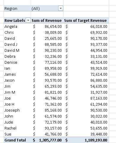
We have created the the Pivot Table and the national sales manager can easily interactively change the filter on the table to focus on the individual regional managers figures.
All good yes?. But the national sales mangers really want each regional manger to have their own report. But that is not a problem!

Create your usual Pivot Table and Region to the report filter.

All we need to do then is hit

• Pivot Table Tools
• Pivot Table
• Options
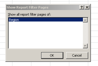
• Show Report Filter Pages

We have one Filter in this Pivot table ….

Select it and then hit Ok.

You will see see all of the Regions now appear in different sheets in your Excel workbook automatically, your national sales ,manager now has all of the reports they need individually to discuss with the regional sales managers.

Job Done!