0:00
today I want to show you how to hide
0:03
negative numbers in your Excel pivot
0:06
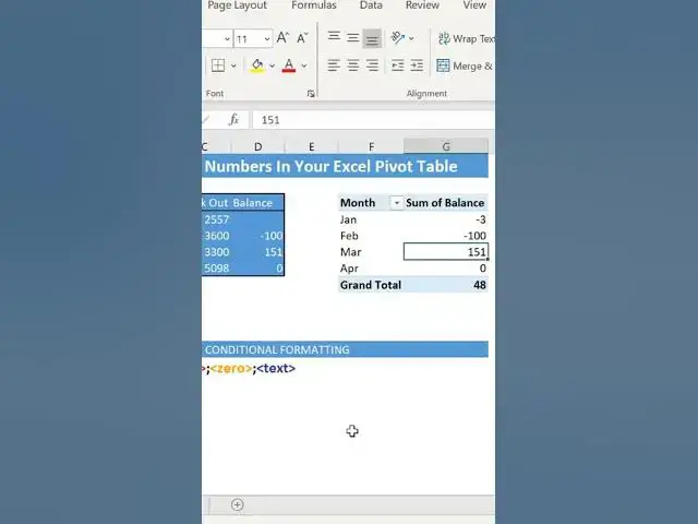
table so I have here a regular pivot
0:09
table and it's based on this data right
0:11
here so as you can see on my pivot I
0:14
have some negative and positive values
0:17
in the stock so what we can do is we can
0:21
use cell formatting to hide the zero and
0:25
the negative numbers so we're only
0:27
showing the positive stock values so
0:29
let's have a quick run through of
0:31
conditional formatting conditional
0:33
formatting has four distinct sections
0:37
for positive numbers negative numbers
0:39
numbers zero and text so if we just go
0:43
into format cells and if we have a look
0:46
at some custom formatting if we wanted
0:49
to show only the positive numbers we
0:52
would type zero if we want to hide the
0:54
negative we use a semicolon
0:58
a semicolon for zero and a semicolon not
1:02
to display text either so now we only
1:05
have the positive number displayed in
1:07
our pivot table a final part of this
1:10
would be I would the grand total doesn't
1:13
show anything of relevance in this so if
1:16
you just go to p pivot table options
1:18
totals and filters I would undo and
1:22
untick grand totals so this just shows
1:25
the positive stock numbers as the grand
1:28
total isn't relative or representative
1:32
in this particular example